Calculus 8: Limits Involving Infinity and Asymptotes

 So far, we have mainly studied limits involving only finite numbers. Here in this lecture note, we discuss limits involving infinity. You may wonder why we want to such limits. They, in fact, do have important applications. One immediate application is that it provides us some information on the shape of a function, i.e. it helps us sketch the graph of a function, as we will see later.

We first begin with the notion of vertical asymptotes.

Definition. The line $x=a$ is called a vertical asymptote of the graph of $y=f(x)$ if $$\lim_{x\to a+}f(x)=\pm\infty,\ \mbox{or}\ \lim_{x\to a-}f(x)=\pm\infty.$$

Example. Find the vertical asymptotes of the graph of $y=\displaystyle\frac{x^2-3x+2}{x^3-4x}$.

Solution. The candidates for vertical asymptotes are the values of $x$ that make the denominator $0$. In our example, they are the root of the equation $x^3-4x=0$. Since $x^3-4x=x(x^2-4)=x(x+2)(x-2)$, we find three roots $x=-2,0,2$. However, some of them may not necessarily be vertical asymptotes. To check this, we calculate the limits: \begin{align*}\lim_{x\to 0+}\frac{x^2-3x+2}{x^3-4x}&=\frac{2}{0-}\ \mbox{(Can you see why?)}\\&=-\infty,\\\lim_{x\to 0-}\frac{x^2-3x+2}{x^3-4x}&=\frac{2}{0+}\\&=\infty,\\\lim_{x\to -2-}\frac{x^2-3x+2}{x^3-4x}&=\frac{12}{0-}\\&=-\infty,\\\lim_{x\to -2+}\frac{x^2-3x+2}{x^3-4x}&=\frac{12}{0+}\\&=\infty,\\\lim_{x\to 2}\frac{x^2-3x+2}{x^3-4x}&=\lim_{x\to 2}\frac{(x-1)(x-2)}{x(x+2)(x-2)}\\&=\lim_{x\to 2}\frac{x-1}{x(x+2)}\\&=\frac{1}{8}.\end{align*}
So, we see that $x=0,-2$ are vertical asymptotes while $x=2$ is not.

Definition. A line $y=b$ is called a horizontal asymptote of the graph of $y=f(x)$ if $$\lim_{x\to\infty}f(x)=b,\ \mbox{or}\ \lim_{x\to -\infty}f(x)=b.$$

Example. Find the horizontal asymptotes of the graph of $y=\displaystyle\frac{5x^2+8x-3}{3x^2+2}$.

Solution. You can notice at once that the limit $\displaystyle\lim_{x\to\infty}\frac{5x^2+8x-3}{3x^2+2}$ is an $\frac{\infty}{\infty}$ type indeterminate form. So how do we calculate this kind of indeterminate form? First divide the numerator and the denominator by the highest power of $x$ appeared in the denominator:\begin{align*}\lim_{x\to\infty}\frac{5x^2+8x-3}{3x^2+2}&=\lim_{x\to\infty}\frac{\frac{5x^2+8x-3}{x^2}}{\frac{3x^2+2}{x^2}}\\&=\lim_{x\to\infty}\frac{5+\frac{8}{x}-\frac{3}{x^2}}{3+\frac{2}{x^2}}\\&=\frac{5}{3}.\end{align*} The final answer is obtained by the limit $\displaystyle\lim_{x\to\infty}\frac{1}{x^n}=0,$ where $n$ is a positive integer.

Similarly, $\displaystyle\lim_{x\to\infty}\frac{5x^2+8x-3}{3x^2+2}=\frac{5}{3}$ using the limit $\displaystyle\lim_{x\to -\infty}\frac{1}{x^n}=0,$ where $n$ is a positive integer. The following picture contains the graphs of the function (in blue) and the horizontal asymptote (in red).

The graph of $y=\frac{5x^2+8x-3}{3x^2+2}

Example. Find the horizontal asymptotes of $y=\displaystyle\frac{x^2-3x+2}{x^3-4x}$.

Solution. The limits $\displaystyle\lim_{x\to\pm\infty}\frac{x^2-3x+2}{x^3-4x}$ is $\frac{\infty}{\infty}$ type indeterminate form. So as we did in the previous example, we first divide the numerator and the denominator by the highest power of $x$ that is appeared in the denominator: \begin{align*}\lim_{x\to\infty}\frac{x^2-3x+2}{x^3-4x}&=\lim_{x\to\infty}\frac{\frac{x^2-3x+2}{x^3}}{\frac{x^3-4x}{x^3}}\\&=\lim_{x\to\infty}\frac{\frac{1}{x}-\frac{3}{x^2}+\frac{2}{x^3}}{1-\frac{4}{x^2}}\\&=0.\end{align*}

Similarly you find that $\displaystyle\lim_{x\to -\infty}\frac{x^2-3x+2}{x^3-4x}=0$.

The following picture shows you the graph of the function (in blue), the horizontal and the vertical asymptotes (in red).

The graph of $y=\frac{x^2-3x+2}{x^3-4x}

Normally the graph of a function $y=f(x)$ never touches or crosses its horizontal asymptote while it gets closer and closer to its horizontal asymptote as $x\to\infty$ or $x\to -\infty$. But there are exceptions as shown in the following example.

Example. Consider the function $f(x)=2+\displaystyle\frac{\sin x}{x}$. Using the Sandwich Theorem, one can show that $\displaystyle\lim_{x\to\pm\infty}\frac{\sin x}{x}=0$ and hence $\displaystyle\lim_{x\to\pm\infty}f(x)=2$. That is $y=2$ is a horizontal asymptote of the curve. As you can see in the following picture, the graph crosses the horizontal asymptote $y=2$ infinitely many times.

The graph of $y=2+\frac{sin(x)}{x}$

The graph of $y=\frac{2x^3-3}{7x+4}$

There is another kind of asymptotes, called oblique (slanted) asymptotes. An oblique asymptote can be seen from a rational function $\frac{p(x)}{q(x)}$ where $\deg p(x)>\deg q(x)$. An oblique asymptote is in fact given by a dominating term of such a rational function as you can see in the following example.

Example. Consider the rational function $f(x)=\displaystyle\frac{2x^2-3}{7x+4}$. By long division, we obtain \begin{align*}f(x)&=\frac{2x^2-3}{7x+4}\\&=\left(\frac{2}{7}x-\frac{8}{49}\right)+\frac{-115}{49(7x+4)}.\end{align*} As $x\to\pm\infty$, the remainder $\displaystyle\frac{-115}{49(7x+4)}\to 0$. Hence the graph of $f(x)$ gets closer to the graph of the linear function $y=\displaystyle \frac{2}{7}x-\frac{8}{49}$ as $x\to\pm\infty$. This linear function is an oblique (slanted) asymptote of the graph of $f(x)$. The following picture shows the graph of $f(x)$ (in blue) and both the vertical asymptote $x=-\frac{4}{7}$ and the oblique asymptote $y=\frac{2}{7}x-\frac{8}{49}$ (in red).

Here is a closer look.

The graph of $y=\frac{2x^3-3}{7x+4}$

Calculus 7: Continuity

Intuitively speaking, we say a function is continuous at a point if its graph has no separation, i.e. there is no hole or breakage, at that point. Such notion of continuity can be defined explicitly as follows.

Definition: A function \(f(x)\) is said to be continuous at a point \(x=a\) if \[\lim_{x\to a}f(x)=f(a).\]

Note that the above definition assumes the existence of both \(\displaystyle\lim_{x\to a}f(x)\) and \(f(a)\).

There are 3 different types of discontinuities.
 

1.  \(f(a)\) is not defined.

Example. Consider the function\[f(x)=\frac{x^2-4}{x-2}.\] Clearly \(f(2)\) is not defined. However the limit \(\displaystyle\lim_{x\to 2}f(x)\) exists:\begin{eqnarray*}\lim_{x\to 2}\frac{x^2-4}{x-2}&=&\lim_{x\to 2}\frac{(x+2)(x-2)}{x-2}\\&=&\lim_{x\to 2}(x+2)=4.\end{eqnarray*} As a result the graph has a hole.

The graph of $f(x)=\frac{x^2-4}{x-2}$

This kind of discontinuity is called a removable discontinuity, meaning that we can extend \(f(x)\) to a function which is continuous at \(x=a\) in the following sense: Define \(g(x)\) by\[g(x)=\left\{\begin{array}{ccc}f(x)\ \mbox{if}\ x\ne a,\\\lim_{x\to a}f(x)\ \mbox{if}\ x=a.\end{array}\right.\]Then \(g(x)\) is a continuous at \(x=a\). The function \(g(x)\) is called the continuous extension of \(f(x)\). What we just did is basically filling the hole and the filling is the limit \(\displaystyle\lim_{x\to a}f(x)\). For the above example, we define\[g(x)=\left\{\begin{array}{ccc}\frac{x^2-4}{x-2} &\mbox{if}& x\ne 2,\\4 &\mbox{if}& x=2.\end{array}\right.\] Then \(g(x)\) is continuous at \(x=2\) and in fact, it is identical to \(x+2\).

2. \(\displaystyle\lim_{x\to a}f(x)\) deos not exist.

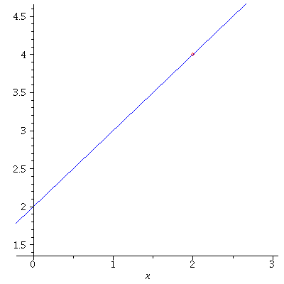
Example. Let \(f(x)=\left\{\begin{array}{cc}2x-2,\ &1\leq x<2\\3,\ &2\leq x\leq 4.\end{array}\right.\) \(f(2)=3\) but \(\displaystyle\lim_{x\to 2}f(x)\) does not exist because \(\displaystyle\lim_{x\to 2-}f(x)=2\) while \(\displaystyle\lim_{x\to 2+}f(x)=3\).

The graph of $f(x)=\left\{\begin{array}{cc}2x-2,\ &1\leq x<2\\3,\ &2\leq x\leq 4\end{array}\right.$

3. \(f(a)\) is defined and \(\displaystyle\lim_{x\to a}f(x)\) exists, but \(\displaystyle\lim_{x\to a}f(x)\ne f(a)\).

Example. Let \(f(x)=\left\{\begin{array}{cc}\displaystyle\frac{x^2-4}{x-2},\ &x\ne 2\\3,\ &x=2.\end{array}\right.\) Then \(f(2)=3\) and \(\displaystyle\lim_{x\to 2}f(x)=4\).

The graph of $f(x)=\left\{\begin{array}{cc}\displaystyle\frac{x^2-4}{x-2},\ &x\ne 2\\3,\ &x=2\end{array}\right.$

From the fundamental limit laws (the first theorem here), we obtain the following properties of continuous functions.

Theorem. If functions \(f(x)\) and \(g(x)\) are continuous at \(x=a\), then

1. \((f\pm g)(x)=f(x)\pm g(x)\) is continuous at \(x=a\).
2. \(f\cdot g(x)=f(x)\cdot g(x)\) is continuous at \(x=a\).
3. \(\displaystyle\frac{f}{g}(x)=\frac{f(x)}{g(x)}\) is continous at \(x=a\) provided \(g(a)\ne 0\).
   

There are some important classes of continuous functions.

• Every polynomial function \(p(x)=a_nx^n+a_{n-1}x^{n-1}+\cdots+a_0\) is continuous everywhere, because \(\displaystyle\lim_{x\to a}p(x)=p(a)\) for any \(-\infty<a<\infty\).
• If \(p(x)\) and \(q(x)\) are polynomials, then the rational function \(\displaystyle\frac{p(x)}{q(x)}\) is continuous wherever it is defined \(\{x\in\mathbb{R}|q(x)\ne 0\}\).
• \(y=\sin x\) and \(y=\cos x\) are continuous everywhere.
• \(y=\tan x\) is continous where it is defined, i.e. everywhere except at the points \(x=\pm\frac{\pi}{2},\pm\frac{3\pi}{2},\pm\frac{5\pi}{2},\cdots\).
• If \(n\) is a positive integer, then \(y=\root n\of{x}\) is continuous where it is defined. That is, if \(n\) is an odd integer, it is defined everywhere. If \(n\) is an even integer,it is defined on \([0,\infty)\), the set of all non-negative real numbers.
  

Recall that the composite function \(g\circ f(x)\) of two functions \(f(x)\) and \(g(x)\) (read \(f\) followed by \(g\)) is defined by \[g\circ f(x):=g(f(x)).\]

Theorem. Suppose that \(\displaystyle\lim_{x\to a}f(x)=L\) exists and \(g(x)\) is a continuous function at \(x=L\). Then\[\lim_{x\to a}g\circ f(x)=g(\lim_{x\to a}f(x)).\]

It follows from this theorem that the composite function of two continuous functions is again a continuous function.

Corollary. If \(f(x)\) is continuous at \(x=a\) and \(g(x)\) is continuous at \(f(a)\), then the composite function \(g\circ f(x)\) is continuous at \(x=a\).

Example. The function \(y=\sqrt{x^2-2x-5}\) is the composite function  \(g\circ f(x)\) of two functions \(f(x)=x^2-2x-5\) and \(g(x)=\sqrt{x}\). The function \(f(x)=x^2-2x-5\) is continuous everywhere while \(g(x)=\sqrt{x}\) is continuous on \([0,\infty)\), so by the preceding corollary, the composite function \(g\circ f(x)=\sqrt{x^2-2x-5}\) is continuous on its domain \((-\infty,1-\sqrt{6}]\cup [1+\sqrt{6},\infty)\). The following picture shows the graph of \(y=\sqrt{x^2-2x-5}\) on \((-\infty,1-\sqrt{6}]\cup [1+\sqrt{6},\infty)\). Notice that $y=\sqrt{x^2-2x-5}$ is a part of the hyperbola $\frac{(x-1)^2}{6}-\frac{y^2}{6}=1$ where $y\geq 0$.

The graph of $y=\sqrt{x^2-2x-5}$

Continuous functions exhibit many nice properties. I would like to introduce a couple of them here. The first is the so-called Max-Min Theorem.

Theorem. [Max-Min Theorem] If \(f(x)\) is a continuous function on a closed interval \([a,b]\), \(f(x)\) attains its maximum value and minimum value on \([a,b]\).

Another important property is the so-called the Intermediate Value Theorem (IVT). The IVT has an important application in the study of equations.

Theorem. [The Intermediate Value Theorem] If \(f(x)\) is continuous on a closed interval \([a,b]\) and \(f(a)\ne f(b)\), then \(f(x)\) takes on every value between \(f(a)\) and \(f(b)\). In other words, if \(f(a)<k<f(b)\) (assuming that \(f(a)<f(b)\)), then \(f(c)=k\) for some number \(a<c<b\).

It follows from the IVT that

Corollary. If \(f(x)\) is continuous on a closed interval \([a,b]\) and \(f(a)\cdot f(b)<0\), then \(f(x)=0\) for some \(a<x<b\).

Using  this corollary we can tell if a root of the equation \(f(x)=0\) can be found in some interval. For instance

Example. Show that the equation \(x^3-x-1=0\) has a root in the interval \([-1,2]\).

Solution. Let \(f(x)=x^3-x-1\). Then \(f(x)\) is continuous on \([-1,2]\). Since \(f(-1)=-1\) and \(f(2)=5\) have different signs, by the preceding corollary there is a root of \(x^3-x-1=0\) in the open interval \((-1,2)\).

Calculus 6: How to Calculate Limits III

 In this lecture note, we discuss limits of trigonometric functions. The most basic trigonometric functions are of course \(y=\sin x\) and \(y=\cos x\). They have the following limit properties.

Theorem. For any \(a\in\mathbb R\), \[\lim_{x\to a}\sin x=\sin a,\ \lim_{x\to a}\cos x=\cos a.\]

You notice that both \(y=\sin x\) and \(y=\cos x\) satisfy the same limit property as polynomial functions as seen here. This is not a coincidence and the reason behind this is that polynomial functions, \(y=\sin x\) and \(y=\cos x\) are continuous functions. This will become clear when we discuss the continuity of a function later. Limit properties of other trigonometric functions stem out of the above theorem along with limit laws discussed here. For example, the limit property of \(y=\tan x\) is given by \[\lim_{x\to a}\tan x=\lim_{x\to a}\frac{\sin x}{\cos x}=\frac{\sin a}{\cos a}=\tan a,\] where \(\tan a\) is defined or equivalently \(\cos a\ne 0\).

Theorem. Suppose that \(f(x)\leq g(x)\) near \(x=a\) and both \(\displaystyle\lim_{x\to a}f(x)\), \(\displaystyle\lim_{x\to a}g(x)\) exist. Then \[\lim_{x\to a}f(x)\leq \lim_{x\to a}g(x).\]

Corollary. [Squeeze Theorem, Sandwich Theorem] Suppose that \(f(x)\leq g(x)\leq h(x)\) near \(x=a\). If \(\displaystyle\lim_{x\to a}f(x)=\lim_{x\to a}h(x)=L\) then \[\lim_{x\to a}g(x)=L.\]

Squeeze Theorem is useful for calculating a certain type of limits such as the following example.

Example. Find the limit \(\displaystyle\lim_{x\to 0}x^2\sin\frac{1}{x}\).

Solution. Since \(-1\leq\sin\frac{1}{x}\leq 1\), \[-x^2\leq x^2\sin\frac{1}{x}\leq x^2\] for all \(x\ne 0\). Since \(\displaystyle\lim_{x\to 0}(-x^2)=\lim_{x\to 0}x^2=0\), by Squeeze Theorem \[\lim_{x\to 0}x^2\sin\frac{1}{x}=0.\] The following picture also confirms our result.

The graph of $y=x^2\sin\frac{1}{x}$

There is another important limit that involves a trigonometric function.  It is

Theorem. \(\displaystyle\lim_{x\to 0}\frac{\sin x}{x}=1\).

This is an important formula. You will readily see that this limit is \(\frac{0}{0}\) type indeterminate form. So this means that \(\sin x\) must have a factor  \(x\) in it. But how do we factor \(\sin x\)? It is not a polynomial! In fact. it is sort of. The function \(\sin x\) is can be written as a never-ending polynomial (such a polynomial is called a power series) \[\sin x=x-\frac{x^3}{3!}+\frac{x^5}{5!}-\frac{x^7}{7!}+\cdots,\]where \(n!\) denotes the \(n\) factorial\[n!=n(n-1)(n-2)(n-3)\cdots3\cdot 2\cdot 1.\] So \begin{align*}\lim_{x\to 0}\frac{\sin x}{x}&=\lim_{x\to 0}\frac{x-\frac{x^3}{3!}+\frac{x^5}{5!}-\frac{x^7}{7!}+\cdots}{x}\\&=\lim_{x\to 0}\left(1-\frac{x^2}{3!}+\frac{x^4}{5!}-\frac{x^6}{7!}+\cdots\right)\\&=1.\end{align*}

We have now confirmed that the formula is indeed correct, but is there a more fundamental proof without using power series? Yes, there is. In fact it can be proved using trigonometry. First consider the case when \(x\to 0+\). In this case, without loss of generality we may assume that \(x\) is an acute angle so we have the following picture.

The areas of \(\triangle OAC\), \(\sphericalangle OBC\) and \(\triangle OBD\) are, respectively, given by \(\frac{1}{2}\cos x\sin x\), \(\frac{1}{2}x\) and \(\frac{1}{2}\tan x\). Clearly from the picture they satisfy the inequality \[\frac{1}{2}\cos x\sin x<\frac{1}{2}x<\frac{1}{2}\tan x.\] Dividing this inequality by \(\frac{1}{2}\sin x\) (note that \(\sin x>0\) since \(x\) is an acute angle) we obtain\[\cos x<\frac{x}{\sin x}<\frac{1}{\cos x}\] or equivalently,\[\frac{1}{\cos x}<\frac{\sin x}{x}<\cos x.\] Now \(\displaystyle\lim_{x\to 0+}\cos x=\lim_{x\to 0+}\frac{1}{\cos x}=1\), so by Squeeze Theorem,\[\lim_{x\to 0+}\frac{\sin x}{x}=1.\] Similarly, we can also show that\[\lim_{x\to 0-}\frac{\sin x}{x}=1.\] Hence this completes the proof.

Example. Find $\displaystyle\lim_{x\to 0}\frac{\sin 7x}{4x}$.

Solution. \begin{align*}\lim_{x\to 0}\frac{\sin 7x}{4x}&=\lim_{x\to 0}\frac{7}{4}\frac{\sin 7x}{7x}\\&=\frac{7}{4}\lim_{x\to 0}\frac{\sin 7x}{7x}\\&=\frac{7}{4}\ \left(\lim_{x\to 0}\frac{\sin 7x}{7x}=1\right).\end{align*}

Example. Find $\displaystyle\lim_{\theta\to 0}\frac{\cos\theta-1}{\theta}$.

Solution. \begin{align*}\lim_{\theta\to 0}\frac{\cos\theta-1}{\theta}&=\lim_{\theta\to 0}\frac{\cos\theta-1}{\theta}\frac{\cos\theta+1}{\cos\theta+1}\\&=\lim_{\theta\to 0}\frac{\cos^2\theta-1}{\theta(\cos\theta+1)}\\&=\lim_{\theta\to 0}\frac{\cos^2\theta-1}{\theta(\cos\theta+1)}\\&=\lim_{\theta\to 0}\frac{-\sin^2\theta}{\theta(\cos\theta+1)}\\&=-\lim_{\theta\to 0}\frac{\sin\theta}{\theta}\frac{\sin\theta}{\cos\theta+1}\\&=-\lim_{\theta\to 0}\frac{\sin\theta}{\theta}\cdot\lim_{\theta\to 0}\frac{\sin\theta}{\cos\theta+1}\\&=-1\cdot 0=0.\end{align*}

Calculus 5: How to Calculate Limits II

In here, we studied how to calculate the limit of a rational function (corollary there). Let us state it here again:

Corollary. [Limit of a Rational Function] Let \(p(x)\) and \(q(x)\) be two polynomials. Then for any real number \(b\), \[\lim_{x\to b}\frac{p(x)}{q(x)}=\frac{p(b)}{q(b)}\] provided \(q(b)\ne 0\).

But what if \(q(b)=0\)? To answer this question let us take a look at the following example.

Example. Find the limit \(\displaystyle\lim_{x\to -1}\frac{x^2+3x+2}{x^2-x-2}\).

Solution. Let \(p(x)=x^2+3x+2\) and \(q(x)=x^2-x-2\). Then \(p(-1)=0\) and \(q(-1)=0\). Since \(q(-1)=0\), we cannot use corollary to calculate the limit. So what do we do? Note that \(p(-1)=0\) and \(q(-1)=0\) means that both \(p(x)\) and \(q(x)\) contains a power of \((x+1)\) in them. Let us factor out the maximum common power of \((x+1)\) from \(p(x)\) and \(q(x)\). Since \(x\to -1\), \(x\ne -1\) i.e. \(x+1\ne 0\). So we can cancel the maximum common power of \((x+1)\) and then calculate limit of the resulting function as \(x\to -1\): \begin{align*}\lim_{x\to -1}\frac{x^2+3x+2}{x^2-x-2}&=\lim_{x\to -1}\frac{(x+1)(x+2)}{(x-2)(x+1)}\\&=\lim_{x\to -1}\frac{x+2}{x-2}\ \mbox{since \(x\ne -1\)}\\&=-\frac{1}{3}.\end{align*}
Remark. [Indeterminate Form] In the above example,
\[\frac{\displaystyle\lim_{x\to -1}(x^2+3x+2)}{\displaystyle\lim_{x\to -1}(x^2-x-2)}=\frac{0}{0}.\] What is this? and how do we understand it? It turns out that the quantity \(\frac{0}{0}\) is not undefined but something else. Remember that here \(0\) is not a number but an infinitesimal, a state that is extremely close to the number \(0\). The quantity \(\frac{0}{0}\) is called an indeterminate form. There are other types of indeterminate forms, to name a few, \(\frac{\infty}{\infty}\), \(0\cdot\infty\), \(0^0\), etc. We will study them later. There are four possibilities for the value of an indeterminate form: \(0\), \(\pm\infty\), or a non-zero real number. Although we denote infinitesimals by the same symbol \(0\), some infinitesimals dominate others. For instance, consider the limit of a rational function \(\displaystyle\lim_{x\to a}\frac{p(x)}{q(x)}\). Suppose that \(\displaystyle\lim_{x\to a}p(x)=\lim_{x\to a}q(x)=0\). There can be three possible scenarios then:

1. If \(p(x)\) approaches \(0\) way faster than \(q(x)\) does, then \(\displaystyle\lim_{x\to a}\frac{p(x)}{q(x)}=0\).
2. If \(q(x)\) approaches \(0\) way faster than \(p(x)\) does, then \(\displaystyle\lim_{x\to a}\frac{p(x)}{q(x)}=\pm\infty\).
3. If \(p(x)\) and \(q(x)\) approaches \(0\) at about the same rate (speed), then \(\displaystyle\lim_{x\to a}\frac{p(x)}{q(x)}\) may be a non-zero real number.
   

Example. Find the limit \[\lim_{x\to 2}\frac{4-x^2}{3-\sqrt{x^2+5}}.\]

Solution. \(\displaystyle\lim_{x\to 2}(4-x^2)=\lim_{x\to 2}(3-\sqrt{x^2+5})=0\). This means that both the numerator and the denominator have a power of \(x-2\) as a common factor. As we did in the previous example, we would attempt to factor both the numerator and the denominator. Only problem is that the denominator is not a polynomial and we don't know how to factor it. Well, we learned about rationalizing the denominator in algebra. We multiply the numerator and the denominator by the conjugate \(3+\sqrt{x^2+5}\) of the denominator. More specifically,\begin{align*}\lim_{x\to 2}\frac{4-x^2}{3-\sqrt{x^2+5}}&=\lim_{x\to 2}\frac{4-x^2}{3-\sqrt{x^2+5}}\cdot\frac{3+\sqrt{x^2+5}}{3+\sqrt{x^2+5}}\\&=\lim_{x\to 2}\frac{(4-x^2)(3+\sqrt{x^2+5})}{4-x^2}\\&=\lim_{x\to 2}(3+\sqrt{x^2+5})\\&=6.\end{align*}

Calculus 4: How to Calculate Limits I

 When you calculate limits, the following theorem plays a crucial role.

Theorem. Suppose that \(c\) is a constant and the limits \[\lim_{x\to a}f(x)\ {\rm and}\ \lim_{x\to a}g(x)\] exist. Then the following properties hold:

1. \(\displaystyle\lim_{x\to a}\{f(x)+g(x)\}=\lim_{x\to a}f(x)+\lim_{x\to a}g(x)\)
2. \(\displaystyle\lim_{x\to a}cf(x)=c\lim_{x\to a}f(x)\)
3. \(\displaystyle\lim_{x\to a}f(x)g(x)=\lim_{x\to a}f(x)\cdot\lim_{x\to a}g(x)\)
4. \(\displaystyle\lim_{x\to a}\frac{f(x)}{g(x)}=\frac{\displaystyle\lim_{x\to a}f(x)}{\displaystyle\lim_{x\to a}g(x)}\) provided \(\displaystyle\lim_{x\to a}g(x)\ne 0\)
   

Before we discuss how to calculate limits, there are very basic limits we need to know. They are: \[\lim_{x\to a}x=a\ {\rm and}\ \lim_{x\to a}c=c,\] where \(c\) is a constant. The limits are trivial from our intuition and also from their graphs. However, those who have analytical mind may want to prove them. They can be proved using the Cauchy's definition of a limit we discussed here. Let us first prove \(\displaystyle\lim_{x\to a}x=a\).

Proof. Let \(\epsilon>0\) be given. Choose \(\delta=\epsilon\). Then for all \(x\) that satisfies the inequality \[|x-a|<\delta,\] it is true that \[|x-a|<\epsilon.\]

Now we prove \(\displaystyle\lim_{x\to a}c=c,\) where \(c\) is a constant.

Proof. Let \(\epsilon>0\) be given. Choose \(\delta>0\) to be any positive real number. Then for all \(x\) that satisfies the inequality \[|x-a|<\delta,\] we have \[|c-c|=0<\epsilon.\]

Using these two limits, we can now show the following useful theorem for calculating limits of polynomial functions.

Theorem. Let \(p(x)\) be a polynomial. Then for any real number \(b\), \[\lim_{x\to b}p(x)=p(b).\]

Proof. Let \(p(x)\) be a polynomial of degree \(n\). Then \(p(x)\) can be written as \[p(x)=a_nx^n+a_{n-1}x^{n-1}+\cdots+a_2x^2+a_1x+a_0,\] where \(a_n,a_{n-1},\cdots,a_2,a_1,a_0\) are constant real coefficients. Now
\begin{align*}
\lim_{x\to b}p(x)&=\lim_{x\to b}(a_nx^n+a_{n-1}x^{n-1}+\cdots+a_2x^2+a_1x+a_0)\\
&=\lim_{x\to b}a_nx^n+\lim_{x\to a}a_{n-1}x^{n-1}+\cdots+\lim_{x\to a}a_2x^2+\lim_{x\to a}a_1x+\lim_{x\to a}a_0,\ (\mbox{property 1})\\
&=a_n\lim_{x\to b}x^n+a_{n-1}\lim_{x\to b}x^{n-1}+\cdots+a_2\lim_{x\to b}x^2+a_1\lim_{x\to b}x+a_0\ (\mbox{property 2 &}\ \lim_{x\to b}a_0=a_0)\\
&=a_nb^n+a_{n-1}b^{n-1}+\cdots+a_2b^2+a_1b+a_0,\ (\lim_{x\to b}x=b\ \&\ \mbox{property 3})\\
&=p(b).
\end{align*}

This theorem also implies that any polynomial function is continuous everywhere. We will discuss the notion of continuity later.

Due to this theorem and property 4 of the previous theorem, the following corollary about the limit of a rational function holds.

Corollary. [Limit of a Rational Function] Let \(p(x)\) and \(q(x)\) be two polynomials. Then for any real number \(b\), \[\lim_{x\to b}\frac{p(x)}{q(x)}=\frac{p(b)}{q(b)}\] provided \(q(b)\ne 0\).

Theorem. [Other Important Limits] Suppose that \(\displaystyle\lim_{x\to a}f(x)\) exists. Then the following properties hold:

1. \(\displaystyle\lim_{x\to a}f(x)^n=[\displaystyle\lim_{x\to a}f(x)]^n\)
2. \(\displaystyle\lim_{x\to a}\root n\of{f(x)}=\root n\of{\displaystyle\lim_{x\to a}f(x)}\)
3. \(\displaystyle\lim_{x\to a}\ln f(x)=\ln[\displaystyle\lim_{x\to a}f(x)]\)
4. \(\displaystyle\lim_{x\to a}\sin f(x)=\sin[\displaystyle\lim_{x\to a}f(x)]\)
5. \(\displaystyle\lim_{x\to a}\cos f(x)=\cos[\displaystyle\lim_{x\to a}f(x)]\)
   

It is assumed that \(\displaystyle\lim_{x\to a} f(x)\) belongs to the domain of each function in each property. For example, in property 2 if \(n\) is an even integer, it is required that \(\displaystyle\lim_{x\to a} f(x)\geq 0\). The first property is a direct consequence of property 3 of the first theorem. The rest of the properties are related to the continuity of a function. This will be discussed later.

Calculus 3: The Precise Definition of a Limit

The definition of a limit we previously discussed here is intuitive and qualitative rather than quantitative. It may be helpful for us to conceptually understand the notion of a limit, but it is useless when you try to prove some fundamental properties of limits, for instance the properties described in the following theorem.

Theorem. Suppose that \(c\) is a constant and the limits \[\lim_{x\to a}f(x)\ {\rm and}\ \lim_{x\to a}g(x)\] exist. Then the following properties hold:

1. \(\displaystyle\lim_{x\to a}\{f(x)+g(x)\}=\lim_{x\to a}f(x)+\lim_{x\to a}g(x)\)
2. \(\displaystyle\lim_{x\to a}cf(x)=c\lim_{x\to a}f(x)\)
3. \(\displaystyle\lim_{x\to a}f(x)g(x)=\lim_{x\to a}f(x)\cdot\lim_{x\to a}g(x)\)
4. \(\displaystyle\lim_{x\to a}\frac{f(x)}{g(x)}=\frac{\displaystyle\lim_{x\to a}f(x)}{\displaystyle\lim_{x\to a}g(x)}\) provided \(\displaystyle\lim_{x\to a}g(x)\ne 0\)
   

For a long time, mathematicians have believed that the above properties were true and have used them without having been able to prove them. A limit is a mathematical quantity and in order to deal with a mathematical quantity, one needs to have a quantitative definition. And a quantitative definition must consist of quantities that are finite. Finally a French mathematician Augustin-Louis Cauchy came up with such a definition.

Definition. [\(\epsilon-\delta\) Argument] A function \(f(x)\) is said to approach a value \(A\) as \(x\) approaches \(a\), if for any given positive number \(\epsilon>0\) (no matter how small it is) there exists a positive number \(\delta>0\) such that \[|f(x)-A|<\epsilon\] is true for every \(x\) that satisfies the inequality \[0<|x-a|<\delta.\]

The following figure illustrates why this definition makes sense.

$\lim_{x\to a}f(x)=A$

Example. Prove that \(\displaystyle\lim_{x\to 2}(5x-2)=8\).

Solution: Let \(\epsilon>0\) be given. Then we want to show that there exists \(\delta>0\) such that \[|(5x-2)-8|=|5x-10|<\epsilon\] is satisfied, whenever \(x\) is in the domain \[0<|x-2|<\delta.\] Now divide the inequality \(|5x-10|<\epsilon\) by \(5\). Then we obtain \[|x-2|<\frac{\epsilon}{5}.\] Hence, \(\delta=\frac{\epsilon}{5}\)is an adequate choice for \(\delta\) and the proof is complete.

If \(\epsilon=0.005\), the preceding result tells us that the function \(5x-2\) will lie in the range \(7.995<5x-2<8.005\) whenever the domain of \(x\) is \(1.999<x<2.001\).

Example. In order to see why the above definition does not work for non-existing limits, let us recall the second example from here: \[f(x)=\left\{\begin{array}{ccc}x-1 & {\rm if} & x<2\\(x-2)^2+3 & {\rm if} & x\geq 2.\end{array}\right.\] Let us show that the left-hand limit \(1\) of \(f(x)\) at \(x=2\) cannot be a limit of \(f(x)\) when \(x\) approaches \(2\). Let \(\epsilon=1\). Then no matter how small \(\delta>0\) one chooses there is a number \(2<x_0<2+\delta\) and \(f(x_0)>3\). That is, \(f(x_0)\) does not satisfy the inequality \(0<f(x)<2\). Hence, \(2\) cannot be a limit. Similarly, one can show that the right-hand limit \(3\) of \(f(x)\) at \(x=1\) cannot be a limit either.

In order to see how the Cauchy's definition of a limit can be used to prove some fundamental properties of limits, we prove the first property of the above theorem: If \[\lim_{x\to a}f(x)=A\ {\rm and}\ \lim_{x\to a}g(x)=B\] then \[\lim_{x\to a}\{f(x)+g(x)\}=A+B.\]

Proof. Let \(\epsilon>0\) be given. Since \(\displaystyle\lim_{x\to a}f(x)=A\) and \(\displaystyle\lim_{x\to a}g(x)=B\), there exist \(\delta_1>0\) and \(\delta_2>0\) such that \[|f(x)-A|<\frac{\epsilon}{2},\] whenever \(0<|x-a|<\delta_1\) and such that \[|g(x)-B|<\frac{\epsilon}{2},\] whenever \(0<|x-a|<\delta_2\). Choose \(\delta=\min(\delta_1,\delta_2)\), i.e. we choose \(\delta\) to be the smaller of \(\delta_1\) and \(\delta_2\). Now if \(x\) satisfies the inequality \[0<|x-a|<\delta\] then
\begin{align*}
|f(x)+g(x)-(A+B)|&=|f(x)-A+g(x)-B|\\
&=\leq |f(x)-A|+|g(x)-B|\\
&<\frac{\epsilon}{2}+\frac{\epsilon}{2}\\
&=\epsilon.
\end{align*}
This completes the proof.

The rest of the properties in the above theorem can be proved in a similar manner. I stumbled upon the Cauchy's definition of a limit back when I was a high school senior. Once I understood what it means, I was so amazed by its beauty. After I proved all the properties listed in the above theorem, I felt some kind of enlightenment. It was a long time ago, but I still remember the joy and the excitement from that little experience. It was an awakening moment for me that opened my eyes to the beauty of the Nature and the Universe. Surely, that experience led me to mathematics. Hope you can experience that too.

Calculus 2: Examples of Non-Existing Limits

The limit of a function does not necessarily exist. Possible cases of non-existing limits may occur when

1. at least one of the one-sided limits does not exist;
2. both one-sided limits exist but they are not the same.
   

Here are a couple of examples of non-existing limits.

Example. Let \(f(x)\) be the function defined by \(f(x)=\sin\frac{1}{x}\) for \(x\ne 0\). The graph of this function is given by 

The graph of $f(x)=\sin\frac{1}{x}$

As \(x\) approaches \(0\), \(\sin\frac{1}{x}\) keeps oscillating near the \(y\)-axis and it does not approach anywhere. This is the case when neither \(\lim_{x\to 0-}\sin\frac{1}{x}\) nor \(\lim_{x\to 0+}\sin\frac{1}{x}\) exists. The following picture shows you a closer look at the graph near the \(y\)-axis.

The graph of $f(x)=\sin\frac{1}{x}$

Example. Let \(f(x)\) be the function defined by \[f(x)=\left\{\begin{array}{ccc}x-1 & {\rm if} & x<2\\(x-2)^2+3 & {\rm if} & x\geq 2.\end{array}\right.\] The graph of \(f(x)\) is

The graph of $$f(x)=\left\{\begin{array}{ccc}x-1 & {\rm if} & x<2\\(x-2)^2+3 & {\rm if} & x\geq 2.\end{array}\right.$$

Let us calculate the left-hand and the right-hand limit of \(f(x)\) at \(x=2\): \begin{align*}\lim_{x\to 2-}f(x)&=\lim_{x\to 2-}(x-1)\\&=1,\\\lim_{x\to 2+}f(x)&=\lim_{x\to 2+}(x-2)^2+3\\&=3.\end{align*} Both the left-hand and the right-hand limits of \(f(x)\) exist, however they do not coincide. Hence the limit \(\lim_{x\to 2}f(x)\) does not exist.

Calculus 1: Limits of Functions

 It is very important for students to get familiar with the notion of a function, some important classes of functions (polynomial functions, rational functions, and trigonometric functions, etc.) and their properties, and trigonometry before they begin to study calculus. If you are not comfortable with some of these, you should brush up on them.

If you have not studied calculus before, you will notice that it is very different from any subject of mathematics you have encountered before. Calculus deals with a notion of closeness or nearness. Imagine that the variable \(x\) does not just represent a fixed number as a solution of an equation but it keeps changing and approaching a number, say \(2\), closer and closer. This describes a state in which \(x\) is very near the number \(2\). Such a state will be denoted by \(x\to 2\). To get some better picture, you may imagine a flying arrow that keeps getting closer and closer to the target but it never hits the target. Such notion of nearness plays a very important role in mathematics and it is developed into topology, one of the most important and fundamental subjects of mathematics. In particular, the state \(x\to 0\) is called infinitesimal and is also denoted by \(0\). Infinitesimal means "extremely small." What would be confusing to students who learn calculus for the first time is that infinitesimal \(0\) and the number \(0\) are denoted by the same symbol. There is a branch of advanced mathematics, so-called non-standard analysis. In there, infinitesimal is treated as a number and is denoted by \(0^\ast\) in order to distinguish it from the number \(0\). But we are not going to use this notation. So how do we distinguish them? It turns out that it is not difficult to distinguish them from the context as we will see later. So there is absolutely no reason for you to panic. For the same reason, we often write \(x\to 2\) by \(2\), however it is very important for you to see it, from the context, as a state in which \(x\) is very near 2, not as the fixed number 2. Using the notations from non-standard analysis, it can be written \(2^\ast=2+0^\ast.\) Before we move on, I would like to point out that there are clear distinctions between an infinitesimal \(0\) and the number \(0\). First, an infinitesimal \(0\) can be positive or negative while the number \(0\) is neutral. A positive infinitesimal and a negative infinitesimal may be represented by the notations \(x\to 0+\) and \(x\to 0-\), respectively. The notation \(x\to 0+\) means that \(x\) is approaching \(0\) from the right (or from above \(0\)). Similarly, \(x\to 0-\) means that \(x\) is approaching \(0\) from the left (or from below \(0\)). Second, one can divide a number by an infinitesimal while the division of a number by the number \(0\) is not defined. For instance, \(\frac{1}{0}\) is not defined when \(0\) is a number but \(\frac{1}{0}=\infty\) when \(0\) is a positive infinitesimal. Similarly, \(\frac{1}{0}=-\infty\) if \(0\) is a negative infinitesimal.

In calculus, we are interested in the behavior of a function near a point. For instance, we want to study how the function \[f(x)=\frac{x^2-1}{x-1}\] behaves near \(x=1\). Note that the function is not defined at \(x=1\). The most direct way to study this is to use sample values of \(x\) that get closer to 1 and see how the values of \(f(x)\) change.
$$
\begin{array}{|c|c|}
\hline
\mbox{Values of \(x\) below and above \(1\)} & \mbox{\(f(x)=\frac{x^2-1}{x-1}\)}\\
\hline
\hline
0.9 & 1.9\\
\hline
0.99 & 1.99\\
\hline
0.999 & 1.999\\
\hline
0.999999 & 1.999999\\
\hline
1.1 & 2.1\\
\hline
1.01 & 2.01\\
\hline
1.001 & 2.001\\
\hline
1.0000001 & 2.0000001\\
\hline
\end{array}
$$

One can guess from the table that the values of \(f(x)=\frac{x^2-1}{x-1}\) approach \(2\) as both \(x\to 1-\) and \(x\to 1+\). In this case, we say that the limit of \(f(x)=\frac{x^2-1}{x-1}\) is \(2\) as \(x\) approaches \(1\) and write \[\lim_{x\to 1}f(x)=2\] or \[\lim_{x\to 1}\frac{x^2-1}{x-1}=2.\] The following graph of \(f(x)=\frac{x^2-1}{x-1}\) also clearly shows this.

The graph of $f(x)=\frac{x^2-1}{x-1}$

In our example, \[\lim_{x\to 1-}\frac{x^2-1}{x-1}=\lim_{x\to 1+}\frac{x^2-1}{x-1}=2.\] The one-sided limits \(\lim_{x\to a-}f(x)\) and \(\lim_{x\to a+}f(x)\) are called, respectively, the left-hand limit and the right-hand limit of \(f(x)\) at \(x=a\). They are not necessarily the same, however for the limit of a function to exist at a point, the left-hand limit and the right-hand limit at that point must coincide.

Definition. We say that the limit \(\lim_{x\to a}f(x)\) exists if both \(\lim_{x\to a-}f(x)\) and \(\lim_{x\to a+}f(x)\) exist and they are the same. The limit \(\lim_{x\to a}f(x)\) is defined to be the value of \(\lim_{x\to a-}f(x)\) (or that of \(\lim_{x\to a+}f(x)\)).

Now we have a picture of what the limit of a function is. The next important question is "how do we find the limit?" if it exists. In practice, we do not try to find the limit of a function as we did in the table for reasons. We could only guess the limit by the method and often it is difficult to make a good guess if the function is a more complicated one. Consequently, in many cases, you cannot be certain that your guess is correct even if you come up with one. The method can sometimes mislead. If limits exist, there are ways to calculate them exactly. In the above example, again \(x\to 1\) means that \(x\) is very near \(1\) but not exactly equal to \(1\). Since \(x\ne 1\),
\begin{eqnarray*}\lim_{x\to 1}\frac{x^2-1}{x-1}&=&\lim_{x\to 1}\frac{(x+1)(x-1)}{x-1}\\&=&\lim_{x\to 1}(x+1)\\&=&2.\end{eqnarray*}
The method of finding exact values of limits can vary depending on the types of functions. We will discuss more about it later.

 

Differentiation of Functions of a Complex Variable 4: Harmonic Functions

Throughout this course, a connected open subset of $\mathbb{C}$ is called a domain. Suppose that a function $f(z)=u(x,y)+iv(x,y)$ is analytic in a domain $\mathcal{D}$. Then $f(z)$ satisfies the Cauchy-Riemann conditions. The Cauchy-Riemann conditions are also called the Cauchy-Riemann equations. Differentiating the Cauchy-Riemann equations with respect to $x$, we obtain
\begin{equation}
\label{eq:cr3}
u_{xx}=v_{yx},\ u_{yx}=-v_{xx}
\end{equation}
Differentiating the Cauchy-Riemann equations with respect to $y$, we also obtain
\begin{equation}
\label{eq:cr4}
u_{xy}=v_{yy},\ u_{yy}=-v_{xy}
\end{equation}
By the continuity of the partial derivatives of $u$ and $v$, we have
\begin{equation}
\label{eq:cr5}
u_{xy}=u_{yx},\ v_{xy}=v_{yx}
\end{equation}
Applying the last set of equations to each of the preceding two sets of equations, we obtain the Laplace equations
\begin{equation}
\label{eq:harmonic}
\begin{aligned}
\Delta u&=u_{xx}+u_{yy}=0\\
\Delta v&=v_{xx}+v_{yy}=0
\end{aligned}
\end{equation}
That is, $u$ and $v$ are harmonic  functions in $\mathcal{D}$.

Example. The function $f(z)=e^{-y}\sin x-ie^{-y}\cos x$ is entire, so both $u(x,y)=e^{-y}\sin x$ and $v(x,y)=-e^{-y}\cos x$ are harmonic in $\mathbb{C}$.

Definition. If two function $u$ and $v$ are harmonic in a domain $\mathcal{D}$ and their first-order partial derivatives satisfy the Cauchy-Riemann conditions throughout $\mathcal{D}$, $v$ is said to be a \emph{harmonic conjugate of $u$}.

Theorem. A function $f(z)=u(x,y)+iv(x,y)$ is analytic in a domain $\mathcal{D}$ if and only if $v$ is a harmonic conjugate of $u$.

Remark. If $v$ is a harmonic conjugate of $u$ in a domain $\mathcal{D}$, it is not necessarily true that $u$ is a harmonic conjugate of $v$ in $\mathcal{D}$ as seen in the following example.

Example. Let us consider $f(z)=z^2=x^2-y^2+i2xy$. Since $f(z)$ is entire, $v(x,y)=2xy$ is a harmonic conjugate of $u(x,y)=x^2-y^2$. However, $u$ cannot be a harmonic conjugate of $v$ since $2xy+i(x^2-y^2)$ is nowhere analytic (it is differentiable only at the origin $(0,0)$).

Example. [Finding a harmonic conjugate of a harmonic function] Let $u(x,y)=y^3-3x^2y$ and let $v(x,y)$ be a harmonic conjugate of $u(x,y)$. Then $u$ and $v$ satisfy the Cauchy-Riemann equations. It follows from the Cauchy-Riemann equation $u_x=v_y$ that $v_y=-6xy$. Integrating $v_y$ with respect to $y$, we obtain
$$v(x,y)=-3xy^2+\phi(x)$$
where $\phi(x)$ is some unknown of $x$. We determine $\phi(x)$ using $u_y=-v_x$: Differentiating $v(x,y)$ with respect to $x$, we have
$$v_x=-3y^2+\phi'(x)$$
Comparing this with
$$-u_y=-3y^2+3x^2$$
we get that $\phi'(x)=3x^2$ and so $\phi(x)=x^3+C$ where $C$ is a constant. Hence, we find a harmonic conjugate of $u(x,y)$
$$v(x,y)=-3xy^2+x^3+C$$
The corresponding analytic function is
$$f(z)=y^3-3x^2y+i(-3xy^2+x^3+C)$$

Differentiation of Functions of a Complex Variable 3: The Cauchy-Riemann Conditions in Polar Coordinates

 Let $x=r\cos\theta$ and $y=r\sin\theta$. A complex-valued function of a complex variable $f(z)=u(x,y)+iv(x,y)$ can be viewed as $f(z)=u(r,\theta)+iv(r,\theta)$ in terms of polar coordinates $(r,\theta)$. Using the chain rule, we obtain
\begin{align*}
\frac{\partial u}{\partial r}&=\frac{\partial u}{\partial x}\frac{\partial x}{\partial r}+\frac{\partial u}{\partial y}\frac{\partial y}{\partial r}\\
&=u_x\cos\theta+u_y\sin\theta\\
\frac{\partial u}{\partial\theta}&=\frac{\partial u}{\partial x}\frac{\partial x}{\partial\theta}+\frac{\partial u}{\partial y}\frac{\partial y}{\partial\theta}\\
&=-u_xr\sin\theta+u_yr\cos\theta
\end{align*}
Similarly, we also obtain
\begin{align*}
v_r&=v_x\cos\theta+v_y\sin\theta\\
v_\theta&=-v_xr\sin\theta+v_yr\cos\theta
\end{align*}
Suppose that $f(z)$ satisfies the Cauchy-Riemann conditions. Then
\begin{align*}
v_r&=-u_y\cos\theta+u_x\sin\theta\\
v_\theta&=u_yr\sin\theta+u_xr\cos\theta
\end{align*}
Hence, we get
\begin{equation}
\label{eq:cr2}
ru_r=v_\theta,\ u_\theta=-rv_r
\end{equation}
This is the Cauchy-Riemann conditions in polar coordinates. Assume that $f(z)=u(r,\theta)+iv(r,\theta)$ satisfies the Cauchy-Riemann conditions in polar coordinates and that the partial derivatives of $u(r,\theta)$ and $v(r,\theta)$ are continuous. Then, in terms of polar coordinates, $f'(z)$ is given by
\begin{equation}
f'(z)=e^{-i\theta}(u_r+iv_r)
\end{equation}

Example.
\begin{align*}
f(z)&=\frac{1}{z}\\
&=\frac{1}{r}(\cos\theta-i\sin\theta)
\end{align*}
So, $u(r,\theta)=\frac{1}{r}\cos\theta$ and $v(r,\theta)=-\frac{1}{r}\sin\theta$. The Cauchy-Riemann conditions in polar coordinates are satisfied as
$$ru_r=-\frac{1}{r}\cos\theta=v_\theta,\ u_\theta=-\frac{1}{r}\sin\theta=-rv_r$$
and the partial derivatives of $u(r,\theta)$ and $v(r,\theta)$ are continuous. Hence, $f'(z)$ exists and
\begin{align*}
f'(z)&=e^{-i\theta}\left(-\frac{1}{r^2}\cos\theta+i\frac{1}{r^2}\sin\theta\right)\\
&=\frac{1}{z^2}
\end{align*}

Differentiation of Functions of a Complex Variable 2: Differentiation Formulas

 If $c$ is a constant complex number, then
\begin{equation}
\frac{dc}{dz}=0
\end{equation}
If $n$ is a positive integer, then
\begin{equation}
\label{eq:powerrule}
\frac{dz^n}{dz}=nz^{n-1}
\end{equation}
This formula is called the power rule and it remains valid when $n$ is a negative integer provided $z\ne 0$.

If $c$ is a constant complex number, then
\begin{equation}
\frac{d[cf(z)]}{dz}=c\frac{df}{dz}
\end{equation}
\begin{align}
\frac{d}{dz}[f(z)+g(z)]&=\frac{df(z)}{dz}+\frac{dg(z)}{dz}\\
\frac{d}{dz}[f(z)g(z)]&=\frac{df(z)}{dz}g(z)+f(z)\frac{dg(z)}{dz}\\
\frac{d}{dz}\left[\frac{f(z)}{g(z)}\right]&=\frac{\frac{df(z)}{dz}g(z)-f(z)\frac{dg(z)}{dz}}{[g(z)]^2}
\end{align}
The first two formulas are the linearity, i.e. the complex differentiation $\frac{d}{dz}$ is linear, the third formula is the product rule or the Leibniz rule, and the fourth formula is the quotient rule.

If $W=g(w)$ and $w=f(z)$, then
\begin{equation}
\label{eq:chain}
\frac{dW}{dz}=\frac{dg}{dw}\frac{dw}{dz}
\end{equation}
This is the chain rule.

Example. $$\frac{d}{dz}(2z^2+i)^5=20z(2z^2+i)^4$$

Differentiation of Functions of a Complex Variable 1: Cauchy-Riemann Conditions

 Consider a complex-valued function $f(z)$ of a complex variable. The derivative $f'(z)$ is defined as
\begin{equation}
\label{eq:diff}
f'(z)=\lim_{\Delta z\to 0}\frac{f(z+\Delta z)-f(z)}{\Delta z}
\end{equation}
$f'(z)$ is also denoted by $\frac{df}{dz}$ . The limit in the above definition is independent of the particular approach to the point $z$. Suppose that $f'(z)$ exists. Let $z=x+iy$ and $f(z)=u(z)+iv(z)$. Then
$$\frac{\Delta f}{\Delta z}=\frac{\Delta u+i\Delta v}{\Delta x+i\Delta y}$$
First, let $\Delta y=0$ and $\Delta x\to 0$. Then
\begin{align*}
\lim_{\Delta z\to 0}\frac{\Delta f}{\Delta z}&=\lim_{\Delta x\to 0}\frac{\Delta u}{\Delta z}+i\frac{\Delta v}{\Delta x}\\
&=\frac{\partial u}{\partial x}+i\frac{\partial v}{\partial x}
\end{align*}
This time, we let $\Delta x=0$ and $\Delta y\to 0$. Then
\begin{align*}
\lim_{\Delta z\to 0}\frac{\Delta f}{\Delta z}&=\lim_{\Delta y\to 0}\frac{\Delta u+i\Delta v}{i\Delta y}\\
&=\lim_{\Delta y\to 0}\frac{\Delta v}{\Delta y}-i\frac{\Delta u}{\Delta y}\\
&=\frac{\partial v}{\partial y}-i\frac{\partial u}{\partial y}
\end{align*}
Since $f'(z)$ exists, the two limits must coincide.
$$\frac{\partial u}{\partial x}+i\frac{\partial v}{\partial x}=\frac{\partial v}{\partial y}-i\frac{\partial u}{\partial y}$$
Hence, we obtain
\begin{equation}
\label{eq:cr}
\frac{\partial u}{\partial x}=\frac{\partial v}{\partial y}, \frac{\partial v}{\partial x}=-\frac{\partial u}{\partial y}
\end{equation}
This is called the Cauchy-Riemann conditions. Conversely, let us assume that Cauchy-Riemann conditions are satisfied. In addition, we also assume that the partial derivatives of $u(x,y)$ and $v(x,y)$ are continuous. For small $\Delta x$ and $\Delta y$, we have
\begin{align*}
\Delta f&\approx df\\
&=\frac{\partial f}{\partial x}\Delta x+\frac{\partial f}{\partial y}\Delta y\\
&=\left(\frac{\partial u}{\partial x}+i\frac{\partial v}{\partial x}\right)\Delta x+\left(\frac{\partial u}{\partial y}+i\frac{\partial v}{\partial y}\right)\Delta y
\end{align*}
Dividing this by $\Delta z$, we obtain
\begin{align*}
\frac{\Delta f}{\Delta z}&\approx\frac{\left(\frac{\partial u}{\partial x}+i\frac{\partial v}{\partial x}\right)\Delta x+\left(\frac{\partial u}{\partial y}+i\frac{\partial v}{\partial y}\right)\Delta y}{\Delta x+i\Delta y}\\
&=\frac{\left(\frac{\partial u}{\partial x}+i\frac{\partial v}{\partial x}\right)+\left(\frac{\partial u}{\partial y}+i\frac{\partial v}{\partial y}\right)\frac{\Delta y}{\Delta x}}{1+i\frac{\Delta y}{\Delta x}}
\end{align*}
By the Cauchy-Riemann conditions, we have
$$\frac{\partial u}{\partial y}+i\frac{\partial v}{\partial y}=i\left(\frac{\partial u}{\partial x}+i\frac{\partial v}{\partial x}\right)$$
Therefore, the derivative $\frac{df}{dz}$ is given by
\begin{equation}
\label{eq:diff2}
\frac{df}{dz}=\frac{\partial u}{\partial x}+i\frac{\partial v}{\partial x}
\end{equation}

Example. If $f(z)$ is differentiable at $z=z_0$, meaning $f'(z_0)$ exists and in some neighborhood of $z_0$, then we say that $f(z)$ is analytic at $z=z_0$.  If $f(z)$ is analytic everywhere in the complex plane $\mathbb{C}$, it is called an entire function.

Example. Let us consider $f(z)=z^2$. Let $z=x+iy$. Then $z^2= x^2-y^2+2xyi$, so $u(x,y)=x^2-y^2$ and $v(x,y)=2xy$.
$$\frac{\partial u}{\partial x}=2x=\frac{\partial v}{\partial y}\ \mbox{and}\ \frac{\partial u}{\partial y}=-2y=-\frac{\partial v}{\partial x}$$
Hence, $f(z)=z^2$ satisfies the Cauchy-Riemann conditions. Since the partial derivatives are continuous, $f'(z)$ exists and
$$f'(z)=\frac{\partial u}{\partial x}+i\frac{\partial v}{\partial x}=2x+2yi$$

Example. Let $f(z)=\bar z=x-iy$. Then $u(x,y)=x$ and $v(x,y)=-y$. Since $\frac{\partial u}{\partial x}=1\ne -1=\frac{\partial v}{\partial y}$, $f(z)=\bar z$ is not differentiable at any $z=z_0$, and so it is nowhere analytic.

Remark. A function $f:\mathbb{C}\longrightarrow\mathbb{C}$ may be viewed as $f:\mathbb{R}^2\longrightarrow\mathbb{R}^2$, a vector-valued function of two real variables. However, the notion of differentiability is different between the two. For example, let us consider $f(z)=|z|^2$. It may be viewed as $f(x,y)=x^2+y^2$. As a real-valued function of two real variables, it is differentiable everywhere since $\frac{\partial f}{\partial x}=2x$ and $\frac{\partial f}{\partial y}=2y$ exist everywhere in $\mathbb{R}^2$. However, as a function of a complex variable, $u(x,y)=x^2+y^2$ and $v(x,y)=0$, so the Cauchy-Riemann conditions are not satisfied unless $x=y=0$. Hence, $f(z)=|z|^2$ is differentiable only at $(0,0)$. It is not analytic at $z=0$ nor anywhere else.

Complex Algebra 2: Exponential Form

We can obtain the exponential form of a complex number using polar coordinates. The exponential form can be very useful from time to time. A complex number $z=x+iy$, in terms of polar coordinates
$$x=r\cos\theta,\ y=r\sin\theta,\ r=\sqrt{x^2+y^2},$$
can be written as
\begin{equation}
\begin{aligned}
z&=r(\cos\theta+i\sin\theta)\\
&=re^{i\theta}
\end{aligned}
\end{equation}
$\theta=\tan^{-1}\frac{y}{x}$ is called the argument. The set of all arguments is denoted by $\arg z$. The principal value of $\arg z$, denoted by $\mathrm{Arg}\ z$, is the unique value $\Theta$ such that $-\pi<\Theta\leq\pi$. Then
\begin{equation}
\arg z=\mathrm{Arg}\ z+2n\pi,\ n=0,\pm1,\pm 2,\cdots
\end{equation}
When $z$ is a negative real number, $\mathrm{Arg}\ z$ has the value $\pi$, not $-\pi$.

Example. The principal argument of $z=-1-i$ is $\Theta=-\frac{3\pi}{4}$ and so
$$\arg z=-\frac{3\pi}{4}+2n\pi$$
where $n=0,\pm 1,\pm 2,\cdots$.

Remark. $\arg z$ may not necessarily be represented by the principal argument. For example, $\arg (-1-i)$ may be written as
$$\arg (-1-i)=\frac{5\pi}{4}+2n\pi, \ n=0,\pm 1,\pm 2,\cdots$$
although $\mathrm{Arg}\ (-1-i)\ne\frac{5\pi}{4}$.

In exponential form, $-1-i$ may be written in exponential form as
$$-1-i=\sqrt{2}\exp\left[i\left(-\frac{3\pi}{4}\right)\right]$$
This is one of infinitely many possibilities for the exponential form of $-1-i$.
$$-1-i=\sqrt{2}\exp\left[i\left(-\frac{3\pi}{4}+2n\pi\right)\right]\ (n=0,\pm 1,\pm2,\cdots)$$

The equation of a circle centered at $z_0$ with radius $R$ is given by
\begin{equation}
\label{eq:circle}
|z-z_0|=R
\end{equation}
In exponential form, the above equation of a circle can be written as
\begin{equation}
\label{eq:circle2}
z=z_0+Re^{i\theta}
\end{equation}
where $0\leq\theta\leq 2\pi$.

Let $z_1=r_1e^{i\theta}$ and $z_2=r_2e^{i\theta_2}$. Then
\begin{align}
\label{eq:product2}
z_1z_2&=r_1r_2e^{i(\theta_1+\theta_2)}\\
\label{eq:quotient}
\frac{z_1}{z_2}&=\frac{r_1}{r_2}e^{i(\theta_1-\theta_2)}
\end{align}
The product and the quotient in exponential form imply the identities.
\begin{align}
\label{eq:arg}
\arg(z_1z_2)&=\arg z_1+\arg z_2\\
\label{eq:arg2}
\arg\left(\frac{z_1}{z_2}\right)&=\arg z_1-\arg z_2
\end{align}
These identities are not necessarily true when $\arg$ is replaced by $\mathrm{Arg}$ as seen in the following example.

Example. Let $z_1=-1$ and $z_2=i$. Then $\mathrm{Arg}\ z_1=\pi$ and $\mathrm{Arg}\ z_2=\frac{\pi}{2}$.
$$\mathrm{Arg}(z_1z_2)=\mathrm{Arg}(-i)=-\frac{\pi}{2}$$
and
$$\mathrm{Arg}\ z_1+\mathrm{Arg}\ z_2=\pi+\frac{\pi}{2}=\frac{3\pi}{2}$$
Thus,
$$\mathrm{Arg}(z_1z_2)\ne \mathrm{Arg}\ z_1+\mathrm{Arg}\ z_2$$

Example. Find the principal argument $\mathrm{Arg}\ z$ when $z=\frac{-2}{1+\sqrt{3}i}$.

Solution.
\begin{align*}
\arg z&=\arg\left(\frac{-2}{1+\sqrt{3}i}\right)\\
&=\arg(-2)-\arg(1+\sqrt{3}i)
\end{align*}
$\mathrm{Arg}(-2)=\pi$ and $\mathrm{Arg}(1+\sqrt{3}i)=\frac{\pi}{3}$. One value of $\arg z$ is $\pi-\frac{\pi}{3}=\frac{2\pi}{3}$. Since $-\pi<\frac{2\pi}{3}\leq\pi$, $\mathrm{Arg}\left(\frac{-2}{1+\sqrt{3}i}\right)=\frac{2\pi}{3}$.

Solution 2. $\frac{-2}{1+\sqrt{3}i}=\frac{-1+\sqrt{3}i}{2}$. So, $\mathrm{Arg}\left(\frac{-2}{1+\sqrt{3}i}\right)=\frac{3\pi}{2}$.

De Moivre's formula
\begin{equation}
\label{eq:demoivre}
(\cos\theta+i\sin\theta)^n = \cos n\theta+i\sin n\theta,\ n=0,\pm 1,\pm2,\cdots
\end{equation}
can be easily proved using the Euler's identity.

Example. Write $(\sqrt{3}+i)^7$ in the form $a+ib$.

Solution. $\sqrt{3}+i=2e^{i\frac{\pi}{6}}$.
\begin{align*}
(\sqrt{3}+i)^7&=(2e^{i\frac{\pi}{6}})^7\\
&=2^7e^{i\frac{7\pi}{6}}\\
&=(2^6e^{i\pi})(2e^{i\frac{\pi}{6}})\\
&=-64(\sqrt{3}+i).
\end{align*}
The exponential form of a complex number can be used to find the $n$-th root of a complex number. Let us consider the complex equation
\begin{equation}
\label{eq:nthroot}
z^n=z_0
\end{equation}
Plugging $z=re^{i\theta}$ and $z_0=r_0e^{i\theta_0}$ into the complex equation results in
$$r^ne^{in\theta}=r_0e^{i\theta_0}$$
Comparing the LHS and the RHS, we obtain
$$r^n=r_0\ \mbox{and}\ n\theta=\theta_0+2k\pi,\ k=0,1,2,\cdots,n-1$$
that is
\begin{equation}
\label{eq:nthroot2}
r=\root n\of{r_0}\ \mbox{and}\ \theta=\frac{\theta_0}{n}+\frac{2k\pi}{n},\ k=0,1,2,\cdots,n-1
\end{equation}
Hence, the $n$-th root of $z_0$ is given by
\begin{equation}
\label{eq:nthroot3}
z=\root n\of{r_0}\exp\left[\frac{i(\theta_0+2k\pi)}{n}\right],\ k=0,1,2,\cdots,n-1
\end{equation}

Example. Find the $n$-th root of unity, i.e. solve the equation
\begin{equation}
\label{eq:nthroot4}
z^n=1
\end{equation}

Solution. It follows from the above $n$-root of $z_0$ formula with $z_0=1$ that
the $n$-th root of unity is given by
\begin{equation}
\label{eq:nthroot5}
\omega_n^k=\exp\left(i\frac{2k\pi}{n}\right),\ k=0,1,2,\cdots,n-1
\end{equation}
The set of the $n$-th root of unity
$$E_n=\{1,\omega_n^1,\omega_n^2,\cdots,\omega_n^{n-1}\}$$
is a cyclic group of  order $n$, which is isomorphic to $\mathbb{Z}_n$. The following figures show beautiful geometric shapes formed by $E_3, E_4, E_5, E_6$.

$E_3$

 

$E_4$

$E_5$

$E_6$

Complex Algebra 1: Complex Numbers

 A complex number is a number of the form $z=x+iy$, where $x,y\in\mathbb{R}$ and $i$ is the number whose square is $-1$. $i$ is called the pure imaginary number. $i$ is symbolically written as $i=\sqrt{-1}$. The real numbers $x$ and $y$ are called, respectively, the real part and imaginary part of $z$ and we also write them as $x=\mathrm{Re}\ z$ and $y=\mathrm{Im}\ z$. Since there is no real number $i$ satisfying $i^2=-1$, it is called an imaginary number. But the number $i$ is as real as any real number. It just does not live in the one-dimensional world (the number line) but actually in two-dimensional world! The set of all complex numbers is denoted by $\mathbb{C}$ and is called the complex plane. It turns out the complex plane can be identified with the real plane $\mathbb{R}^2$ via the map
$$x+iy\in\mathbb{C}\longmapsto (x,y)\in\mathbb{R}^2$$
Notice that under this identification, $i=(0,1)$. This identification is topological, i.e. $\mathbb{C}$ is homeomorphic to $\mathbb{R}^2$. From an algebraic point of view, however, $\mathbb{C}$ and $\mathbb{R}^2$ are different. As we will see, $\mathbb{C}$ with operations $+$ and $\cdot$ is an algebraic structure called a field but $\mathbb{R}^2$ is not.

Complex Plane versus Real Plane

Let $z_1=x_1+iy_1$ and $z_2=x_2+iy_2$ be two complex numbers. They also can be represented as ordered pairs as $z_1=(x_1,y_1)$ and $z_2=(x_2,y_2)$. Two complex numbers $z_1$ and $z_2$ are equal if and only if $x_1=x_2$ and $y_1=y_2$. The sum of two complex numbers $z_1$ and $z_2$ is defined by
\begin{equation}
\label{eq:sum}
z_1+z_2=x_1+x_2+i(y_1+y_2)
\end{equation}
The multiplication $z_1\cdot z_2$ is defined by
\begin{equation}
\label{eq:product}
\begin{aligned}
z_1\cdot z_2&=(x_1+iy_1)(x_2+iy_2)\\
&=x_1x_2-y_1y_2+i(x_1y_2+x_2y_1)
\end{aligned}
\end{equation}
The addition $+$ is associative and commutative. $0$ is the additive identity and for each $z\in\mathbb{C}$, $-z$ is an  additive inverse. This means that $(\mathbb{C},+)$ is an abelian group. The multiplication $\cdot$ is associative and commutative. $1$ is the multiplicative identity and for each nonzero complex number $z=x+iy$, there is a multiplicative inverse $\frac{1}{z}$.
\begin{equation}
\label{eq:inverse}
\begin{aligned}
\frac{1}{z}&=\frac{1}{x+iy}\\
&=\frac{x-iy}{(x+iy)(x-iy)}\\
&=\frac{x}{x^2+y^2}-i\frac{y}{x^2+y^2}
\end{aligned}
\end{equation}
This means that $(\mathbb{C}\setminus\{0\},\cdot)$ is an abelian group. There are also distributive laws hold in usual sense. In this case, we say $(\mathbb{C},+,\cdot)$ is a field.

For $z=x+iy$, $\bar z=x-iy$ is called the conjugate of $z$. As seen above,
\begin{equation}
\begin{aligned}
z\bar z&=x^2+y^2\\
&=(\mathrm{Re}\ z)^2+(\mathrm{Im}\ z)^2
\end{aligned}
\end{equation}
and clearly,
\begin{equation}
\bar{\bar z}=z
\end{equation}
The norm, length, or modulus of $z$ is defined by
\begin{equation}
\begin{aligned}
|z|&=\sqrt{z\bar z}\\
&=\sqrt{(\mathrm{Re}\ z)^2+(\mathrm{Im}\ z)^2}\\
&=\sqrt{x^2+y^2}
\end{aligned}
\end{equation}

Example.
\begin{align*}
|-3+2i|&=\sqrt{(-3+2i)(-3-2i)}\\
&=\sqrt{9+4}=\sqrt{13}
\end{align*}

Proposition [Triangle Inequality].
\begin{equation}
|z_1+z_1|\leq |z_1|+|z_2|
\end{equation}

Proof. Left as an exercise.

Corollary.
\begin{equation}
||z_1|-|z_2||\leq |z_1+z_2|
\end{equation}

Proof. Left as an exercise.